Electrostatic MACE

We introduce MACE-POLAR-1, a new family of foundation models that extends the MACE architecture with explicit long-range electrostatics. MACE-POLAR-1 augments local atomic energies with a non-self-consistent polarisable field formalism, learning atomic charge and spin densities — represented as multipole expansions in a Gaussian-type orbital basis — directly from energy and force labels alone. Global charge and spin constraints are enforced through learnable Fukui equilibration functions, enabling the model to handle arbitrary charge and spin states and respond to external electric fields, while providing physically interpretable spin-resolved charge densities.

The models are trained on the OMol25 dataset comprising 100 million structures at the ωB97M-V hybrid DFT level of theory. Two variants are available: MACE-POLAR-1-M (medium, 12 Å receptive field) and MACE-POLAR-1-L (large, 18 Å receptive field).

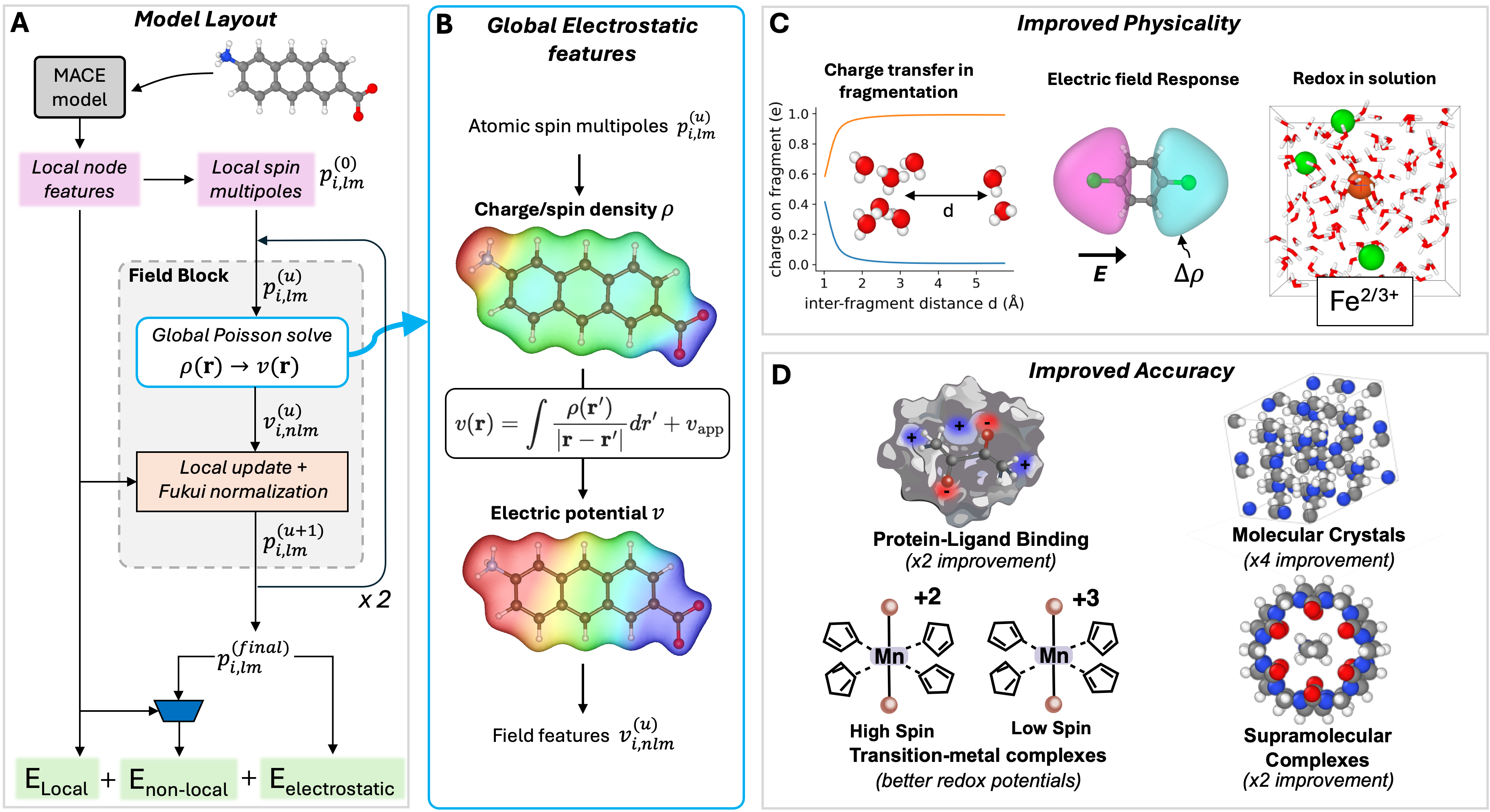
PolarMACE architecture and capabilities overview — Overview of the PolarMACE model layout, global electrostatic features, improved physicality, and improved accuracy across benchmark tasks.

Architecture Summary

PolarMACE keeps the local MACE backbone for short-range chemistry and adds a non-self-consistent long-range update on spin-resolved atomic multipoles. Each update builds non-local electrostatic features from a smooth multipolar density, predicts local multipole corrections, then applies global Fukui equilibration to enforce total charge and spin. The final energy is the sum of local, explicit electrostatic, and learned non-local terms.

Installation

Electrostatic MACE currently requires the latest main branch of MACE and is not supported by the PyPI mace-torch release yet. Install MACE from source first, then install the electrostatics dependency:

git clone https://github.com/ACEsuit/mace.git
cd mace
git checkout main
pip install .
pip install git+https://github.com/WillBaldwin0/graph_electrostatics.git

graph_electrostatics provides the Python module namespace graph_longrange, which PolarMACE requires at runtime.

Available Checkpoints

polar-1-s — small
polar-1-m — medium
polar-1-l — large

Basic Inference

Use the dedicated mace_polar loader, which handles model type and path resolution automatically:

from mace.calculators import mace_polar

calc = mace_polar(
    model="polar-1-m",
    device="cpu",           # or "cuda"
    default_dtype="float64" # use float32 for faster MD
)

atoms.info["charge"] = 0
atoms.info["spin"] = 1
atoms.info["external_field"] = [0.0, 0.0, 0.0]
atoms.calc = calc

energy = atoms.get_potential_energy()
forces = atoms.get_forces()
stress = atoms.get_stress()

Reading Dipole and Charge Density

# populate calc.results
_ = atoms.get_potential_energy()

Energy and Forces

Energies and forces are accessed in the usual ASE way via atoms.get_potential_energy() and atoms.get_forces().

Total Dipole

mu = calc.results["dipole"]  # shape (3,)

The total dipole is only a well-defined quantity for non-periodic systems. For periodic systems it is a meaningless value and should be ignored.

Partial Charges and Partial Dipoles

MACE-POLAR-1 stores atom-centered multipole coefficients as the final values of \(p^{lm}_i\) (spherical multipoles, Condon–Shortley phase convention):

# full multipole array, shape (n_atoms, 4)
p = calc.results["density_coefficients"]

# atomic monopole charges
atomic_charges = p[:, 0]

# cartesian atomic dipoles (px, py, pz)
atomic_dipoles = p[:, [3, 1, 2]]

Note

Partial charges and partial dipoles are not uniquely defined quantities. Furthermore, sums of these quantities over clusters or molecules are also not well defined in general. The only exception is summing over isolated fragments, where isolated means the fragment does not come within approximately 6 Å of any other atom.

Partial Spins

For models with spin support, a spin-resolved multipole array is also available:

# shape (n_atoms, 2, 4) — two spin channels, each with 4 multipole coefficients
p_spin = calc.results["spin_charge_density"]

# spin-up and spin-down atomic charges
charges_up   = p_spin[:, 0, 0]
charges_down = p_spin[:, 1, 0]

The sum across the two spin channels (axis 1) recovers the total density_coefficients array above.

Fine-tuning from Polar Foundation Checkpoints

Use --foundation_model="polar-1-m" or --foundation_model="polar-1-l" with --model="PolarMACE" in mace_run_train.

mace_run_train \
  --name="polar_ft_1m" \
  --model="PolarMACE" \
  --foundation_model="polar-1-m" \
  --train_file="train.xyz" \
  --valid_fraction=0.05 \
  --energy_key="REF_energy" \
  --forces_key="REF_forces" \
  --stress_key="REF_stress" \
  --loss="weighted" \
  --stress_weight=0.0 \
  --force_mh_ft_lr=True \
  --default_dtype="float64" \
  --device="cpu"